Plate-fin heat-sink CHT validation

This study validates FluxCore for conjugate heat-transfer (CHT) simulation of an air-cooled rectangular-fin heat sink. Seven operating points are compared with published measurements and the SimScale reference solution.

Download the original validation report

1. Introduction

Effective thermal management is essential to the performance and service life of electronic components. Air-cooled plate-fin heat sinks remain widely used because they combine simple, manufacturable geometry with a large heat-transfer area and low operating cost. Their apparent simplicity conceals a strongly coupled thermal-fluid problem: heat must spread from a small electronic package through the heat-sink base and fins before being removed by forced airflow. Fin efficiency, developing boundary layers, narrow inter-fin passages and flow bypass all influence the resulting junction temperature and overall thermal resistance [1].

The objective is to demonstrate that FluxCore reproduces the coupled conduction and forced-convection behaviour of a representative electronics cooling assembly, rather than only the fluid flow or solid temperature field in isolation. The target case is based on the experimental characterisation and thermal model reported by Ventola et al. [1].

The benchmark consists of a power transistor mounted beneath an extruded aluminium plate-fin heat sink in a forced-air duct. Seven operating points span the tested range of approach velocity, inlet temperature and dissipated power. For each condition, FluxCore predicts the coupled air velocity and temperature fields, conduction through the device and heat sink, and the junction temperature.

The primary validation quantity is the junction-to-air thermal resistance:

\[R_{ja}=\frac{T_j-T_a}{P}\]

where $T_j$ is device junction temperature, $T_a$ is inlet-air temperature and $P$ is applied device power. Results are compared with the published experimental values and SimScale reference solution.

This is a demanding CHT benchmark because the solution must preserve heat flux across multiple solid-fluid interfaces while resolving large differences in material conductivity, a compact heat source, one-millimetre fins, 2.1 mm fin spacing, wake development and bypass flow around an unshrouded heat sink. Small errors in interface coupling, near-wall resolution or flow distribution can produce a measurable change in $T_j$ and $R_{ja}$. The published geometry, material properties and seven experimental operating points make the case reproducible and provide a direct, quantitative test of FluxCore’s multi-region CHT capability.

2. Simulation setup

2.1 Geometry and computational domain

The geometry follows the SimScale reconstruction [2] of the commercial heat sink tested by Ventola et al. [1]. The extruded-aluminium heat sink is 57.2 mm long and 41.4 mm wide, with a base thickness of 8.4 mm. Fourteen rectangular fins are each 21.8 mm high and 1.0 mm thick, with 2.1 mm clear spacing between adjacent fins.

The heat source represents an STMicroelectronics STP130NS04ZB power transistor. Its modelled envelope is 15.5 × 10 × 4.5 mm and the contact area with the heat sink is 1.555 cm².

The heat sink and device are placed within an air enclosure. Measured from the heat sink, the inlet section extends $6L$ upstream and the outlet section extends $15L$ downstream, where $L=57.2$ mm is the heat-sink length. A symmetry plane through the longitudinal centreline is used for the fluid, heat sink and device, so only half of the physical assembly is simulated. This retains the relevant fin-channel, wake and bypass-flow physics while reducing computational cost [2].

2.2 Computational mesh

The validation mesh was generated using Gradient Dynamics’ structured electronics-meshing workflow. It contains 3,005,974 cells:

• 1,859,477 cells in the fluid region

• 1,146,497 cells in the solid regions

This study records the mesh used for the published comparison. Current Studio production meshing is based on the prism–octree workflow described in the Studio meshing guide.

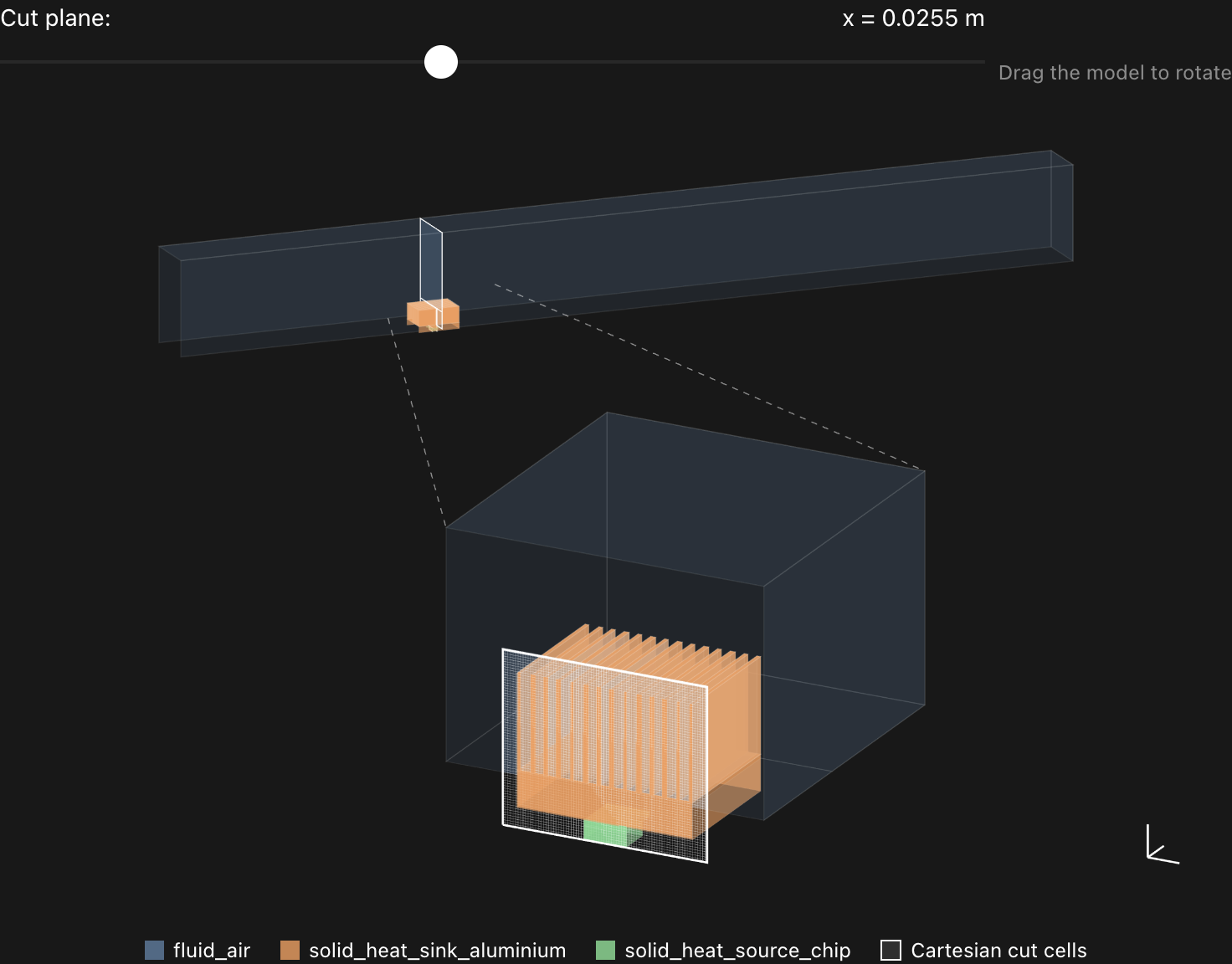
Figure 1. Computational domain, material regions and mesh slice through the heat-sink assembly.

2.3 Materials and thermal coupling

Air is assigned the following properties:

Property	Value
Density	1.179 kg/m³
Kinematic viscosity	$1.529\times10^{-5}$ m²/s
Specific heat capacity	1013 J/(kg·K)
Thermal-expansion coefficient	$3.43\times10^{-3}$ K⁻¹
Laminar Prandtl number	0.713
Turbulent Prandtl number	0.85
Reference temperature	273.1 K

Solid properties follow the SimScale reference model [2]:

Region	Thermal conductivity	Specific heat capacity	Density
Aluminium heat sink	209 W/(m·K)	897 J/(kg·K)	2700 kg/m³
Power device	38.6 W/(m·K)	705 J/(kg·K)	2330 kg/m³

The device conductivity is the effective value used in the SimScale model to represent the manufacturer’s junction-to-case resistance of 0.5 K/W over the stated contact area [2]. At the coupled device-to-sink and sink-to-air interfaces, temperature and normal heat flux are continuous. This allows the calculation to capture heat spreading through the base, conduction along the fins and convective removal by the air in one energy-conserving CHT model.

2.4 Boundary conditions

Each case is run to a steady thermal and flow state. A uniform volumetric-flow inlet is prescribed with the corresponding inlet temperature; the downstream boundary is a 0 Pa gauge-pressure outlet. All solid surfaces exposed to the air are no-slip walls, the centre plane is a symmetry boundary and external enclosure walls are adiabatic. The specified power is applied to the device as the heat input.

2.5 Operating points

The seven conditions reproduce the SimScale rectangular-fin validation matrix [2].

Case	Approach velocity (m/s)	Volumetric flow (m³/s)	Inlet temperature (K)	Device power (W)
1	5.47	0.02700	296.9	56.64
2	7.03	0.03520	297.4	71.40
3	8.59	0.04295	297.9	82.36
4	9.96	0.04980	298.3	87.32
5	11.23	0.05620	298.9	85.07
6	12.50	0.06200	299.3	76.30
7	13.57	0.06783	299.6	60.24

3. Results

FluxCore results are compared with the experimental measurements and SimScale reference across all seven operating points. Figures 2 and 3 show junction temperature and junction-to-air thermal resistance as functions of approach velocity. Figures 4 and 5 show representative velocity and temperature fields.

3.1 Junction temperature

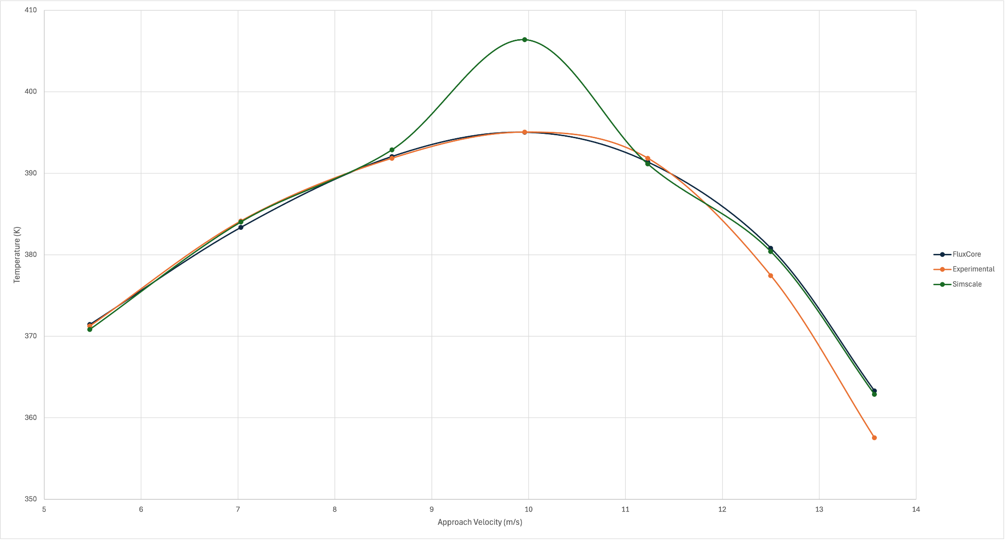
Figure 2. Junction temperature versus approach velocity.

FluxCore reproduces the non-monotonic junction-temperature response and tracks the experimental curve closely from 5.47 to 11.23 m/s, including the peak near 10 m/s. Unlike the SimScale result, which shows a pronounced overprediction at this operating point, FluxCore remains close to the measured value. At 12.50 and 13.57 m/s, FluxCore predicts higher junction temperatures than the experiment, although it remains close to SimScale.

3.2 Junction-to-air thermal resistance

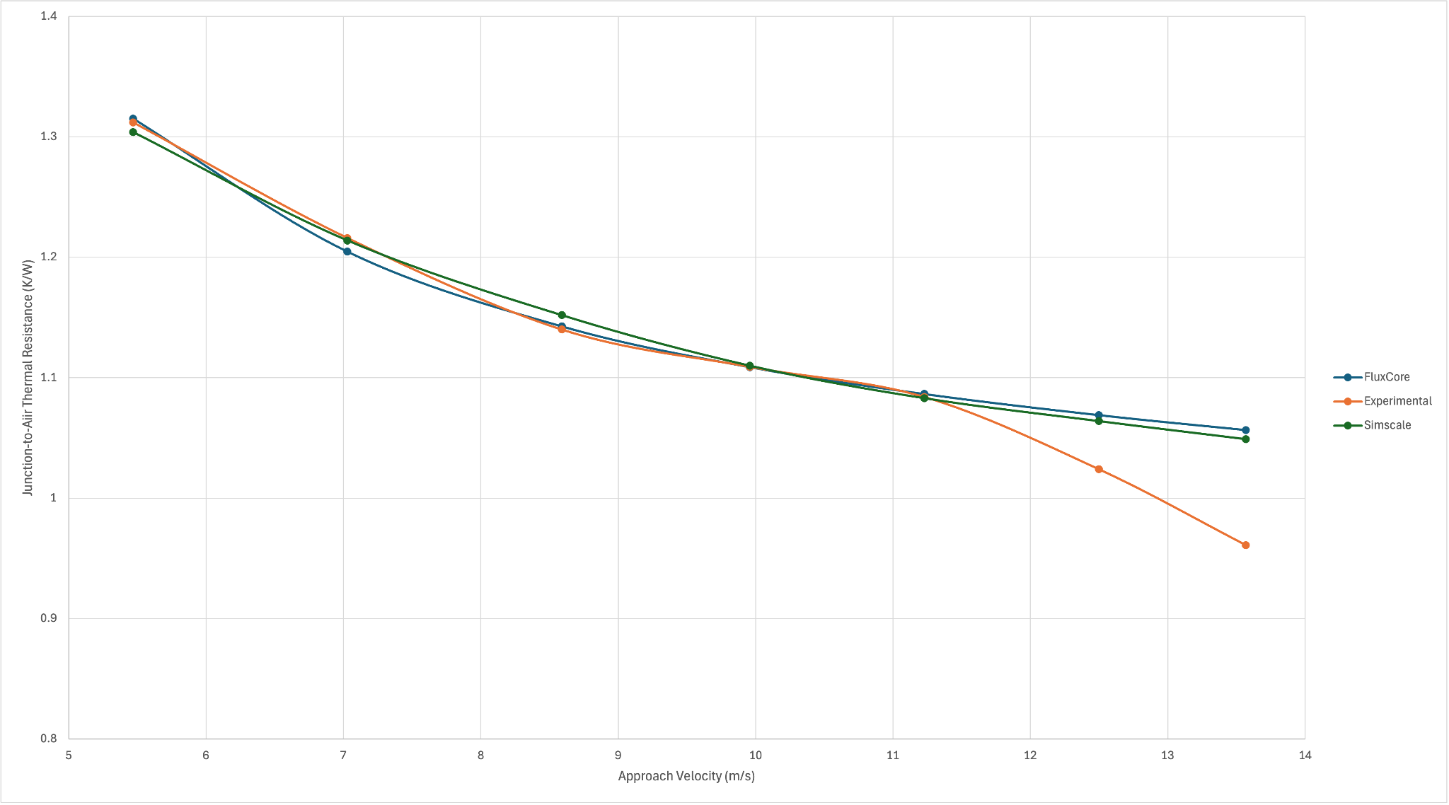
Figure 3. Junction-to-air thermal resistance versus approach velocity.

FluxCore captures the expected reduction in $R_{ja}$ as airflow increases and agrees closely with the experiment over the first five operating points. The largest departures occur at 12.50 and 13.57 m/s, where both CFD solutions remain close to one another but exceed the experimental resistance. The common departure at these points identifies the high-flow regime as the priority for sensitivity checks on boundary conditions, unmodelled heat-loss paths, material properties and mesh resolution.

3.3 Flow and temperature fields

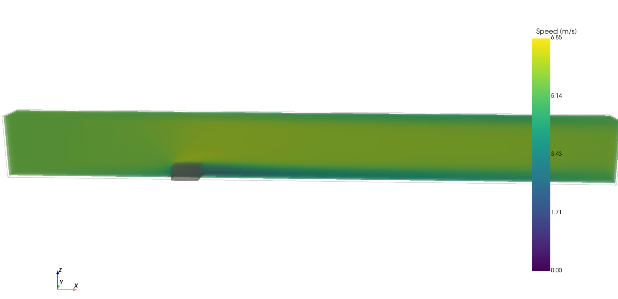
Figure 4. Velocity magnitude on a two-dimensional slice through the domain.

Figure 5. Temperature on a two-dimensional slice through the domain.

The field plots are consistent with the integrated results. The velocity slice shows the flow accelerating around the heat-sink region and a lower-speed wake downstream. The temperature slice shows heat localised around the device and base before being carried downstream in a decaying thermal plume. These features indicate that the solution couples solid conduction, forced convection and downstream heat transport in the expected manner.

4. Summary

FluxCore reproduces the published thermal response of the rectangular-fin heat sink across the seven operating points. It captures the measured junction-temperature peak near 10 m/s and the decrease in junction-to-air thermal resistance with increasing airflow, with close agreement over the low-to-intermediate velocity range.

At the two highest velocities, FluxCore and SimScale remain mutually consistent but both predict higher resistance and junction temperature than the experiment. Overall, the results support FluxCore’s capability for steady multi-region CHT simulations involving localised heat generation, conduction through multiple solids and forced-air cooling, while clearly identifying the high-flow regime as the main area for further validation.

References

1. Ventola, L., Curcuruto, G., Fasano, M., Fotia, S., Pugliese, V., Chiavazzo, E. and Asinari, P. (2016). Unshrouded Plate Fin Heat Sinks for Electronics Cooling: Validation of a Comprehensive Thermal Model and Cost Optimization in Semi-Active Configuration. Energies, 9(8), 608.

2. SimScale GmbH. Validation Case: Conjugate Heat Transfer — Rectangular Fins. Last updated 8 February 2026.